Introduction to RBF's

This article is intended for readers who needs introductory course on basic concepts of RBF interpolation. This article is not description of ALGLIB RBF functions. These functions are described in more details in another article, which we recommend to anyone who want to use ALGLIB package for scattered multidimensional interpolation/fitting. Here we review general concepts, considering ALGLIB features just for comparison.

Problem types

Interpolation problems can be separated into two main classes: problems with spatial variables (XYZ) and problems with mixed, spatial/temporal variables (XY-T). In the problems of the first kind all variables have same dimensions (spatial) and scale. In the problems of the second kind one variable (time) has special meaning, dimension (temporal) and scale. Fundamental limitation of all RBF methods is that they can successfully solve only problems of the first kind.

For example, consider an interpolation problem for a scalar grid in 2D space. There is a set of sensors which measure field magnitude with particular frequency. Average distance between sensors is 1m, average measurement interval is 1ms. Problem of the first kind is to build RBF model which described field state at some moment of time, using only measurements performed at the same time. Problem of the second kind is to describe evolution of the field in time, having a set of time series (measurements performed by sensors at different moments of time).

If you try to solve second problem, you will see that spatial and temporal variables have different scale. RBF is a basis function with radial symmetry, it has same span in all dimensions. Thus, either basis function radius will be equal to 1.0 - ideal for spatial interpolation, but too large for interpolation in time, or it will be equal to 0.001 - ideal for temporal interpolation, but too small to build good spatial model.

In theory, problem can be rescaled. However, optimal scaling coefficients are problem-specific, and there is not out-of-box solution for problems with mixed variables. This limitation is a intrinsic property of the RBF models. Many other interpolation methods, like multidimensional polynomials or splines, are invariant with respect to scaling of the variables. Such methods correctly work when different variables has different scale.

Basis functions

RBF model has following form: f(x)=SUM(w_i·φ(|x-c_i|)). Here φ is a basis function, w_i are weight coefficients, c_i are interpolation centers. Interpolation centers usually coincide with original (input) grid, basis function is usually chosen from the list below, and weights are calculated as solution of the linear system. Following basis functions are used:

• f(r)=exp(-r²/R0²) – Gaussian basis function. The main benefit of this function is that it is compact - it is small at distances about 3·R0 from the center. At distances equal to 6·R0 or larger this function can be considered zero. As result, we have to solve linear system with sparse matrix. However, significant drawback is that we have one parameter to tune - R0. Too small R0 will make model sharp and non-smooth, and too large one will result in system with ill-conditioned matrix.
• f(r)=sqrt(1+(r/R0)²) – multiquadric basis function. Non-compact basis function, which is non-zero at any point. It is very important drawback - we have to solve systems with dense matrices. Another drawback - again, we have to tune R0.
• f(r)=r^2k·ln(r), f(r)=r^2k+1 – polyharmonic basis functions. Non-compact basis functions without tunable parameters. This is the most important advantage of polyharmonic basis. However, non-compactness, its main drawback, very often makes this basis unsuitable for medium and large scale problems. Linear systems with large dense matrices are hard to solve.

ALGLIB implementation of RBF functions uses Gaussian basis. Compactness of the basis functions gives us high performance. We have to tune scale parameter R0, but from our point of view this drawback is insignificant when compared with ability to solve problems with tens and hundreds of thousands points.

Choosing good radius

What does model radius means?

If we choose Gaussian basis function, we have to choose its tunable parameter - radius. Radius R0 sets scale at which basis function is significantly non-zero. Gaussian basis function has its maximum at r=0 (equal 1), it is approximately 0.36 at r=R0, it is approximately 0.02 at r=2·R0, it is approximately 0.0001 at r=3·R0. At distance r=6·R0 or larger Gaussian basis function is indistinguishable from zero.

Another meaning of this parameter is a size of the "spheres of influence" of the points with known function values. Model value at x is determined by function values at nearby nodes, mostly by ones at distance R0 or closer.

One more meaning of this parameter is a typical size of the "gap" in the grid, which can be "repaired" by RBF model. Consider evaluation of the RBF model at some point x, where function value is unknown If there are exists several nodes at distance R0 or closer, model will reproduce original function with good precision. Best results are achieved when x is located between nodes, in the inner part of the interpolation area. However, if nearest nodes are located at distances about 2·R0, then x won't be covered by their basis functions, and model quality at x will be low.

The larger radius we choose, the better will be RBF model. However, large radius usually means large condition number of the system, large error in the coefficients, slow model construction and evaluation. Smaller radius means small error in the coefficients, models which are quick to build and to evaluate. However, radius which is too small leads to rapid degradation of the model quality.

1D example

Consider 1-dimensional RBF interpolation problem. We have equidistant grid of 11 points with known function values, with unit step (red markers). We built three RBF models with different radii, and plotted them at charts below. Lets compare quality of these models.

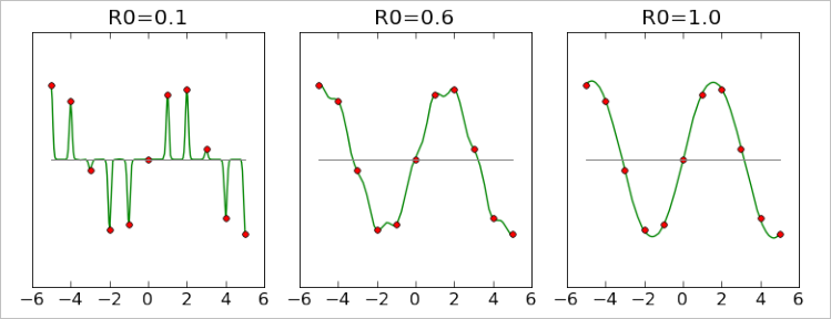
First model was built with radius 0.1, ten times smaller than distance between points. You may see that it passes exactly through all points, but its behavior between them makes it useless. Second model has R0=0.6 and it is significantly better than the first one. However, there is some degree of non-smoothness, sometimes it is clearly biased toward zero ("default value" for RBF models). Third model, which has R0=1 (equal to distance between points) gives almost perfect result.

Note #1
We have not considered interpolation with larger radii, because charts which correspond to R0 > 1 are visually indistinguishable from one built with R0=1.

From charts above we can conclude that radius should be at least equal to the average distance between points d_avg, and for safety reasons it is better to have radius which is several times larger than d_avg. Smaller radii lead to rapid degradation of the model. However, it is important to remember that large radius means larger condition number. Straightforward attempt to solve linear system will face problems with precision even at quite moderate R=3.

2D example

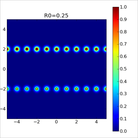
Above we've considered quite simple example - one dimension, equidistant points. It was very simple to choose appropriate radius. Below we consider more complex example: points are located in 2D space at two nearby lines - y=-2 and y=+2. At each of these lines we have equidistant grid with unit step. Distance between lines is four times larger than the grid step, and it complicates radius selection.

We've started from obviously insufficient radius R0=0.25. On the chart below we've plotted model values at each point of the 2D space. You may see that each point (black circle) has "sphere of influence" - colored bubble, which dissolves in the blue background (corresponds to zero, "default value" of the model, which is returned when there is no nearby nodes). However, these spheres do not overlap, model is almost zero in the gaps between them. This chart is a 2D analog of the first of 1-dimensional charts above.

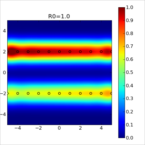
With R0=1 we got new chart (below). "Spheres of influence" grew larger and overlap with each other (red/yellow/green lines at the top and bottom). We can conclude that this model is a good description of the function as long as we stay near y=-2 or y=+2. However, between these two lines there is a part of space which is not covered by the basis functions. At these points, marked by blue color, our model will return zero value.

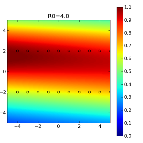
Third chart was built with R0=4 (which is equal to distance between y=-2 and y=+2). This model is many times better than previous ones, because it reproduces function both at y=-2/y=+2 and between them. You may see that basis functions covers space between any pair of points.

Conclusions

From the first example we can conclude that radius should be at least equal to average distance between nodes. Smaller values will give us sharp model which does not reproduce function behavior between nodes. However, average distance is only a lower bound - such radius selection rule works only when space is uniformly filled with nodes. In case there exists non-uniformity, some complex pattern in the distribution of nodes, then "average distance to the nearest neighbor" may be too small for good radius, which was shown by the second example. In the general case radius R0 should so large that for any point where we want to evaluate model there will be several nodes at distance R0 (or closer) around evaluation point.

Polynomial term

We can add linear term to the "basic" RBF model considered above: f(x)=SUM(w_i·φ(|x-c_i|)) + a^T·x+b. Presence of the linear term helps to reproduce global behavior of the function. Instead of linear term we can use polynomial term of the higher degree. From the other side, sometimes better option is to use constant term.

ALGLIB implementation of RBF allows to use linear term, constant term or zero term.

Intermediate results

Above we've studied several choices which arise when we work with RBF models. We can get different models with different properties by choosing different basis functions, polynomial terms and smoothing. There are exists several "popular" models with their own names:

• "classic RBF" — compact basis functions or multiquadrics, no smoothing, optional polynomial term.
• polyharmonic splines - polyharmonic basis functions, no smoothing, polynomial term (essential part of the spline)
• Thin Plate Splines – f(r)=r²·ln(r) is used as basis function, nonlinearity penalty, polynomial term

All these algorithms, albeit known under different names, are just special cases of same general idea - representation of the model function as linear combination of the radially-symmetric basis functions f(r).

Model construction

After choice of the basis function (and, optionally, polynomial term) we have to build model, i.e. to calculate weight coefficients. There exists several approaches to the solution of this problem:

• "straightforward" approach — solution of the linear system using dense solver. It works with any basis function, but we have to live with low performance (solution time grows with number of points N as O(N³). Thus, several thousand of points is a limit for this approach.
• for compact (Gaussian) basis functions we can use sparse linear solver, either direct or iterative one. In this case matrix of the system will be sparse (the more compact basis function we choose, the more sparse matrix we will get). Because convergence of the iterative solver depends on the system conditioning, it will easily solve problems with small radius (approximately equal to the distance till the nearest neighbor), but will have difficulties with larger radii. From the other side, it does not need additional memory. Direct solver can solve problems with larger radii (up to 2-3 distances), but needs additional memory to store LU or Cholesky decomposition of the system.
• in case non-compact basis functions (polyharmonic functions or multiquadrics) are used, linear system will be dense. Direct dense solver will show better results that iterative one, but there exists complex strategy which allows to achieve good performance with iterative solver. In order to accelerate convergence it is possible to use special kind of preconditioning - approximate cardinal basis functions (ACBF) preconditioning. In this case we compose several non-local basis functions to build another, local one (cardinal basis function). It would be great to have perfect local basis with unit condition number, but in reality we have to limit ourselves by some approximate solution (that's why it is called "approximate"). In the new basis our problem can be solved within 5-10 iterations of GMRES solver. Usually, solution itself needs only minor fraction of the total processing time, and most time is spent in the construction of new basis.
• ACBF-preconditioning, which was described above, can be used for compact basis functions too. In this case compact functions become "more compact", which allows us to use iterative solvers with quite large radius, equal to 2 distances till the nearest neighbor.
• another solution which works only with compact basis functions is to separate original dataset into several smaller datasets. RBF construction problem is solved separately for these smaller parts, and then we compose partial models into larger, global one. Model composition is imperfect and we have artifacts near boundaries, so we have to solve interpolation problem one more time - now to correct errors of the first model. As result, we got iterative algorithms, which repeats "separate-solve-compose-correct" loop several times before achieving desired accuracy.
• algorithms described above share one common trait - they solve original problem without any modifications. However, by slightly changing problem statement we can get good interpolant with many times lower performance penalty. For example, instead of N Gaussian functions with same radii we can use more functions with different radii. Interpolation problem can be solved in several steps, by building hierarchy of finer and finer model with decreasing radii. Such approach has several names: hierarchical RBF, multiscale RBF, multilevel RBF or multilayer RBF. Its main benefit - high performance, which achieved due to use of hierarchy of easy to build models.

ALGLIB package implements two approaches to the RBF interpolation: 1) multilayer RBF's with compact basis functions, 2) traditional RBF's with compact basis and ACBF preconditioning.

Model evaluation

After construction of the RBF model we have to solve one more problem: to evaluate model at given point x. Depending on the specific choice of the basis functions (compact or non-compact), two approaches to the evaluation are possible:

• summation of all N basis function, "default" solution which can be used with any basis function. And it is the only solution which is possible for non-compact basis functions.
• summation of nearby basis functions, which are non-zero at the evaluation point. This option can be used only with compact basis functions, and its main benefit is high performance. Such solution requires data structures which support efficient spatial queries, like kd-trees.

ALGLIB package implements second solution: we send a query to kd-tree and generate list of nearby nodes, which are used to calculate function value. Furthermore, ALGLIB include specialized function which efficiently evaluates RBF model on the regular grid - rbfgridcalc2.

Resume

Above we've studied RBF interpolation, basic concepts and subtle tricks, which are used to acvhieve better precision or performance. One particular implementation of the idea above is an ALGLIB package, which:

• uses compact basis functions.
• can solve both interpolation and fitting/smoothing problems.
• includes two RBF algorithms - multiscale RBF's and traditional RBF's with ACBF-preconditioning. In order to accelerate algorithm, efficient sparse LSQR solver is used.
• uses efficient algorithms to accelerate model evaluation (including specialized algorithm for efficient evaluation on regular 2D grids)

We have not studied ALGLIB implementation of RBF's in more details. Those who want to know more can read an article on ALGLIB implementation of RBF's, which contains description of algorithms and comparison of ALGLIB implementation with other packages.

This article is licensed for personal use only.