Fast RBF interpolation/fitting

Scattered multidimensional interpolation is one of the most important - and hard to solve - practical problems. Another important problem is scattered fitting with smoothing, which differs from interpolation by presence of noise in the data and need for controlled smoothing.

Very often you just can't sample function at regular grid. For example, when you sample geospatial data, you can't allocate measurement points as you wish - some places at this planet are hard to reach. However, you may have many irregularly located points with known function values. Such irregular grid may have structure, points may follow some pattern - but it is not rectangular, and it makes impossible to apply two classic interpolation methods (2D/3D splines and polynomials).

ALGLIB package offers you two versions of improved RBF algorithm. ALGLIB implementation of RBF's uses compact (Gaussian) basis functions and many tricks to improve speed, convergence and precision: sparse matrices, preconditioning, fast iterative solver, multiscale models. It results in two distinguishing features of ALGLIB RBF's. First, N·log(N) time complexity - orders of magnitude faster than that of closest competitors. Second, very high accuracy, which is impossible to achieve with traditional algorithms, which start to lose accuracy even with moderate R. Algorithms implemented in ALGLIB can be used to solve interpolation and fitting problems, work with 2D and 3D data, with scalar or vector functions.

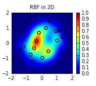
Below we assume that reader is familiar with basic ideas of the RBF interpolation. If you haven't used RBF models before, we recommend you introductory article, which studies basic concepts of RBF models and shows some examples.

Overview of the ALGLIB RBF's

rbf subpackage implements two RBF algorithms, each with its own set of benefits and drawbacks. Both algorithms can be used to solve 2D and 3D problems with purely spatial coordinates (we recommend you to read notes on issues arising when RBF models are used to solve tasks with mixed, spatial and temporal coordinates). Both algorithms can be used to model scalar and vector functions.

First algorithm, RBF-ML, can be used to solve two kinds of problems: interpolation problems and smoothing problems with controllable noise suppression. This algorithm builds multiscale (hierarchical) RBF models. The fact that compact (Gaussian) basis is used allows to achieve O(N·logN) working time, which is orders of magnitude better than O(N³) time (typical for traditional RBF's with dense solvers). Multilayer models allow to: a) use larger radii, which are impossible to use with traditional RBF's; b) reduce numerical errors down to machine precision; c) apply controllable smoothing to data; d) use algorithm both for interpolation and fitting/smoothing. Finally, this algorithm requires minor tuning, but it is robust and won't break in case you've specified too large radius.

The main benefit of the second algorithm, RBF-QNN, is its ability to work without tuning at all - this algorithm uses automatic radius selection. However, it can solve only interpolation problems, can't work with noisy problems, and require uniform distribution of interpolation nodes. Thus, it can be used only with special grids with approximately uniform (although irregular) distribution of points.

RBF-ML interpolation algorithm

Description

RBF-ML algorithm has two primary parameters: initial radius RBase and layers count NLayers. Algorithm builds a hierarchy of models with decreasing radii:

• at 0-th (optional) iteration algorithm builds linear least squares model. Values predicted by linear model are subtracted from function values at nodes, and residual vector is passed to the next iteration.
• at first iteration we build traditional RBF model with radius equal to RBase (usually, RBase is several times larger than the distance between nodes). However, we do not use dense solver and do not try to solve problem exactly. We solve problem in the least squares sense and perform fixed number (about 50) of the LSQR iterations. Usually it is enough to get first, approximate model of the target function. Additional iterations won't improve situation because with such large radius linear system is ill-conditioned. Values predicted by the first layer of the RBF model are subtracted from the function values at nodes. And again, we pass residual vector to the next iteration.
• at each of the subsequent iterations radius is halved, we perform same fixed number of LSQR iterations, and subtract predictions of new models from the residual vector. As result, we have hierarchy of RBF models with different radii, from initial RBase to final RBase·2^-(NLayers-1).
• at first and subsequent iterations we use minor regularization (about 10^-4...10^-3), because it improves convergence of the LSQR solver. Higher values of the regularization coefficient may help us to reduce noise in data. Another way of controlled smoothing is to choose appropriate number of layers. However, we'll consider smoothing in more details in subsequent sections of our article.

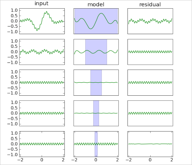
Let's show how our algorithm works on simple 1D interpolation problem. Chart below visualizes model construction for f(x)=exp(-x²)·sin(πt)+0.1·sin(10πt). This function has two components: low-frequency one (first term) and high-frequency one (second term). We build model at interval [-2,+2] using 401 equidistant point and 5-layers RBF model with initial radius RBase=2.

One row of the chart corresponds to one iteration of the algorithm. Input residual is shown at the left, current model is shown in the middle, right column contains output residual ("input residual" - "current model"). Vertical blue bar in the center has width equal to the current RBF radius. Original function can be found at the upper left subchart (input residual for the first iteration).

You may see that at each iteration we build only approximate, inexact models with non-zero residual. Models are inexact because we stop LSQR solver after fixed number of iterations, before solving I-th exactly. However, RBF model becomes more flexible with decrease of basis function radius, and reproduces smaller and smaller features of the original function. For example, low-frequency term was reproduced by two first layers, but high frequency term needed five layers.

Such algorithm has many important features:

• because we use compact basis functions, we have to solve linear systems with sparse matrices, which accelerates LSQR solver. Assuming that radius and density of nodes are constant (i.e. there is approximately constant number of points in the random circle with radius equal to 3·RBase), model construction time depends on number of points N as N·logN. It is many times faster than O(N³) performance typical for straightforward implementations of RBF's.
• iterative algorithm (subsequent layers correct errors of the previous ones) make model robust even with very large initial radius. Problems with large RBase are hard to solve exactly because of ill-conditioning, but subsequent layers will have smaller radii, and well be able to correct inexactness introduced by the first layer.
• use of LSQR solver, which can work with rank deficient matrices, allows us to solve problems with non-distinct nodes in the least squares sense.
• multilayer model allows us to control smoothing both by varying regularization coefficient and by varying number of layers. As we decrease number of layers, we make model less flexible, so it is less prone to noise in data.

Algorithm tuning

RBF-ML algorithm has three tunable parameters: initial radius RBase, number of layers NLayers, regularization coefficient LambdaV.

When you solve interpolation problems, we recommend you to:

• set small non-zero LambdaV, about 10^-4...10^-3 in magnitude (this coefficient is automatically scaled depending on the problem, so same values of LambdaV will give you same regularization independently of the input data). Such minor regularization won't decrease precision of the interpolant (given enough layers, model will fit all points exactly even with non-zero λ), but it will help LSQR solver to converge faster.
• choose large enough initial radius RBase, so it will be able to provide good coverage of the interpolation area by basis functions. It should be several times larger than average distance between points d_avg. Good value to start from - RBase=4·d_avg. Task of finding good initial radius is studied in more details in the corresponding section of the introductory article on RBF interpolation (we recommend to read this section because it contains analysis of the typical errors). We should note that too large RBase will significantly decrease performance (two-fold increase of radius leads to four-fold increase of model construction time), but it won't cause algorithm to fail.
• choose such number of layers NLayers that radius of the final layer r=RBase·2^-(NLayers-1) will be at least two times smaller than d_avg. You may use following formula to determine appropriate number of layers: NLayers=round(ln(2·RBase/d_avg)/ln(2))+2. Such choice guarantees that model will be flexible enough to exactly reproduce input data.

If you want to suppress noise in data, you may choose between two ways of smoothing: smoothing by regularization and smoothing by choosing appropriate number of layers. It is better to use both tricks together:

• choose appropriate initial radius, which provides good coverage of the interpolation area (see recommendations for interpolation problems)
• choose number of layers which provides desired smoothing
• use regularization coefficient for fine control over smoothing

Functions and examples

RBF-ML algorithm is provided by rbf subpackage of the Interpolation package. In order to work with this algorithm you can use following functions:

• rbfcreate - for initialization of the model object (after initialization it contains zero model)
• rbfsetalgomultilayer - to choose RBF-ML as model construction algorithm
• rbfsetconstterm, rbfsetlinterm, rbfsetzeroterm - to choose polynomial term (linear term, constant term, zero term)
• rbfsetpoints - to add dataset to the model
• rbfbuildmodel - to build model using current dataset and algorithm settings
• rbfcalc, rbfcalc2, rbfcalc3, rbfcalcbuf - to evaluate model at given point
• rbfgridcalc2 - to evaluate model at regular 2D grid
• rbfserialize, rbfunserialize - to serialize/unserialize model
• rbfunpack - to unpack model (get RBF centers and radii)

ALGLIB Reference Manual includes several examples on RBF models:

• rbf_d_qnn - QNN algorithm, demonstration of basic concepts (we recommend you to study this example before proceeding to RBF-ML)
• rbf_d_ml_simple - simple example of RBF-ML algorithm
• rbf_d_ml_ls - RBF-ML algorithm solves least squares problem
• rbf_d_polterm - working with polynomial term
• rbf_d_serialize - serialization
• rbf_d_vector - working with vector functions

Comparison with SciPy

In this section we will study performance of the RBF-ML algorithm and compare it with traditional RBF's implemented in the wide-known SciPy package. Following test problem will be solved:

• N points form approximately square Sqrt(N)*Sqrt(N) grid. Points are placed near the nodes of the equidistant grid with unit step, with small pseudorandom offset (about 0.05 in magnitude). In case Sqrt(N) is not integer, we round it to the nearest integer. Function values are pseudorandom in the [-1,+1] range. After generation of the grid, points are randomly reordered.
• SciPy package is represented by scipy.interpolate.Rbf, ALGLIB package is represented by RBF-ML.
• we test different N's from 100...3000, and different RBase from {1.0, 1.5, 2.0, 3.0, 4.0, 5.0}. Here unit radius is approximately equal to the average distance between points.
• SciPy implementation of RBF builds model with fixed radius RBase. ALGLIB implementation of RBF builds model with initial radius RBase and number of layers chosen as NLayers=round(ln(2·RBase)/ln(2))+2 (such choice guarantees that radius of the final layer will be smaller than 1.0).
• following metrics are compared: 1) model construction time, 2) model error at the nodes, 3) memory requirements.
• testing was performed on AMD Phenom II X6 1090T 3.2 GHz, under 64-bit Ubuntu.

First test

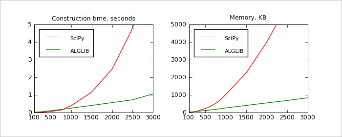
During first test we've solved sequence of problems with RBase=2.0 (moderate radius which gives good precision and robustness) and different N's from [100,3000]. Results can be seen on chart above. We've compared two metrics: model construction time (seconds) and memory usage (KB). Our results allows us to conclude, that:

• for moderate N's (up to 300-600) SciPy implementation of RBF's is faster than that of ALGLIB. However, difference in performance is not striking.
• SciPy package can be used only when N is smaller than 1000. For larger N's we see rapid growth of the model construction time and memory requirements. Construction time grows as O(N³), memory usage - as O(N²).
• ALGLIB package is orders of magnitude faster than SciPy for N≥1000). Construction time grows as O(N·logN), memory requirements - as O(N).
• although not shown on the charts above, but for R=2.0 both algorithms built model with good precision (near the machine ε).
• we have not compared algorithms for larger N's because for N=4000 SciPy RBF become too slow, and for N=5000 SciPy failed to build model. In the independent tests ALGLIB implementation of RBF's successfully solved problem with 100000.

It is important that results above were calculated for one specific radius - RBase=2.0. Below we'll study performance metrics for different values of RBase given fixed N.

Second test

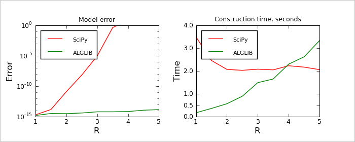
During second test we solved a sequence of problems with fixed N=2000 and different radii from [1.0,5.0]. We used two performance metrics to compare algorithms: 1) model error at the nodes (difference from desired values, which should be fitted exactly) and 2) model construction time. Problems with large radius are hard to solve for both algorithms, but SciPy and ALGLIB face different issues. SciPy implementation of RBF's have problems with ill-conditioning of the linear system, it can't find RBF coefficients with desired precision. ALGLIB implementation of RBF have no problems with precision, but its performance decreases because number of non-zero coefficients in the sparse matrix grows with growth of R. Looking at the charts above, we can conclude that:

• SciPy RBF's can be used only with small values of R. Large R's, starting from R=3.0, make SciPy RBF's useless because of rapid degradation of model quality. SciPy performance is mostly independent from R, but quality rapidly decreases as R grows.
• ALGLIB package can be used for any R, although with different performance. ALGLIB quality is independent from R, but performance decreases quadratically as R grows. Charts do not show results for R > 5, but there are no reasons why ALGLIB can't be used for larger R.
• for N=2000 ALGLIB performance starts to lose the battle with SciPy only at R=4.0, i.e. at the point where SciPy is already useless. Thus, for N≥2000 ALGLIB outperforms SciPy in all situations: either you can't use SciPy because of its low performance, or you can't use it because of its numerical errors. However, it is possible that for N≤2000 and moderate R ALGLIB will be a bit slower than SciPy.
• when we compare performance, we should take into account that SciPy working time grows as O(N³), but ALGLIB working time grows slower - as O(N·logN). Thus, for larger N's difference in performance will be even more striking.

Conclusions

Taking into account information above, we can say that:

• unlike SciPy, ALGLIB RBF's can be used for interpolation with any number of points N (up to 100000) and any R.
• in most situations, ALGLIB shows better performance and better precision than that of SciPy
• SciPy can be successfully used only for small N's (up to 1000) and small R's (up to 2.5). Within its area of expertise SciPy can compete with ALGLIB, and for N≤600 it can outperform ALGLIB. However, outside of this area SciPy faces either breakdown of the model (large R) or significant decrease of performance (large N).

RBF-QNN interpolation algorithm

Distinguishing feature of the RBF-QNN algorithm is its radius selection rule. Instead of one fixed radius, same for all points, it chooses individual radii as follows: radius for each point is equal to distance to nearest neighbor (NN), multiplied by scale coefficient Q (small number between 1.0 and 2.0). Algorithm builds single-layer model, but uses same tricks as RBF-ML: sparse matrices, fast iterative solver. In order to increase convergence, it uses ACBF-preconditioning (approximate cardinal basis functions), which allows to solve problem in less than 10 iterations of the solver. Actually, most of the time is spent in the preconditioner calculation.

As with RBF-ML, RBF-QNN working time grows as O(N·logN). However, unlike RBF-ML, RBF-QNN can't build multilayer models, can't work with radii larger than 2.0, and can't solve problems in the least squares sense (noisy problems, problems with non-distinct nodes, etc.). Core limitation of the algorithm is that it gives good results only on grids with approximately uniform distribution of nodes. Not necessarily rectangular, but nodes must be separated by approximately equal space, and their distribution must be approximately uniform (without clusters or holes). It limits RBF-QNN algorithm by problems with special grids. From the other side, main benefit of such algorithm is its ability to work without complex tuning - radius is selected automatically, algorithm adapts itself to the density of the grid.

RBF-QNN algorithm is used in the same way as RBF-ML. The only difference is that before building RBF model from sample you have to call rbfsetalgoqnn function, which sets RBF-QNN as model construction algorithm.

Conclusion

We've studied two RBF algorithms - RBF-ML and RBF-QNN.

RBF-ML algorithm is a significant breakthrough in the RBF interpolation. It can solve interpolation and smoothing problems, can work with very large datasets (tens of thousands of points) and radii - so large that other algorithms will refuse to work. The most important feature is its high performance - model construction time for N points grows as O(N·logN). RBF-ML can work with arbitrary distribution of nodes, including badly separated or non-distinct nodes. This algorithm is recommended by us as "default solution" for RBF interpolation.

RBF-QNN algorithm was developed as automatically tunable solution, which can be used on a special kind of problems - problems with grid of approximately uniformly distributed nodes. This algorithm is less universal than RBF-ML, but in many cases it can be more convenient.

This article is licensed for personal use only.