Neural networks

Neural networks are one of the most flexible and powerful data mining methods. They can solve regression, classification, prediction problems. Neural networks have been successfully applied in many areas - from financial models to medical problems.

ALGLIB package includes one of the best neural networks on the market: many different architectures, efficient training algorithms, built-in support for cross-validation. All these features are present in both editions - Commercial and Free - of ALGLIB.

Both Free and Commercial editions can solve same set of computational problems. Commercial Edition, however, includes such performance-related features as optimized SSE-capable code (for x86/x64 users) and multithreading support. These features are absent in Free Edition.

This article reviews neural features of the ALGLIB package and evaluates performance of different ALGLIB editions (C++ vs C#, Commercial vs Free).

ALGLIB neural networks

Different architectures

ALGLIB supports neural networks without hidden layers, with one hidden layer, and with two hidden layers. "Shortcut" connections from the input layer directly to the output layer are not supported.

Hidden layers have one of the standard sigmoid-like activation functions, however, a larger variety may be available to the output layer of a neural network. The output layer can be:

• linear (such networks are used in approximation tasks)
• linear with SOFTMAX-normalization
• sigmoid-like, bounded from above AND from below (network output is mapped to specified range [a,b])
• bounded from above OR from below. The simplest case is when this function is tends to x when x tends to +∞, and exponentially tends to zero when x tends to -∞.

Neural networks with a linear output layer and output SOFTMAX-normalization make up a special case. These are used for classification tasks, where network outputs should be nonnegative, and their sum should be strictly equal to one, permitting using them as the probability that the input vector will be referred to one of the classes. The number of outputs in such a network is always no less than two (which is a restriction imposed by the elementary logic).

Such a set of architectures, in spite of being minimalistic, is sufficient to solve most of practical problems. One can concentrate on the problem (classification or approximation), without paying unreasonable attention to details (e.g., the selection of a specific hidden layer activation function usually has little effect on the result).

Rich functionality

ALGLIB offers rich neural functionality. These functions include automatic normalization of data, regularization, training with random restarts, cross-validation.

Data preprocessing is normalization of training data - inputs and output are normalized to have unit mean/deviation. Preprocessing is essential for fast convergence of the training algorithm - it may even fail to converge on badly scaled data. ALGLIB package automatically analyzes data set and chooses corresponding scaling for inputs and outputs. Input data are automatically scaled prior to feeding network, and network outputs are automatically unscaled after processing. Preprocessing is done transparently to user, you don't have to worry about it - just feed data to training algorithm!

Regularization (AKA weight decay) is another important feature implemented by ALGLIB. Properly chosen decay coefficient greatly improves both generalization error and convergence speed.

Training with restarts is a way to overcome problem of bad local minima. On highly nonlinear problems training algorithm may converge to network state which is locally optimal (i.e. can not be improved by small steps), but is very far from the best solution possible (sub-optimal). In such cases you may want to perform several restarts of the training algorithm from random positions, and choose best network after training. ALGLIB does it automatically and allows you to specify desired number of restarts prior to training.

Cross-validation is a well known procedure for producing estimates of the generalization error without having separate test set. ALGLIB allows to perform cross-validation with just one single call - you specify number of folds, and package handles everything else.

High performance

Both editions of ALGLIB (Free and Commercial) include advanced training methods with many algorithmic improvements. In addition to that, Commercial Edition includes following important optimizations: multithreading, SSE intrinsics (for C++ users), optimized native core (for C# users).

ALGLIB can parallelize following operations: dataset processing (data are split into batches which are processed separately), training with random restarts (training sessions corresponding to different starting points can be performed in different threads), cross-validation (parallel execution of different cross-validation rounds). Parallel neural networks can work on any multicore system - from x86/x64 to SPARC and ARM processors! Multi-processor systems are supported too. Neural networks are easily parallelizable, so you should expect almost linear speed-up from going parallel!

Another improvement present in Commercial Edition of ALGLIB for C++ is SSE support, which can be very useful to x86/x64 users. SIMD instructions allow us to accelerate processing of small microbatches.

Finally, in C# version of ALGLIB Commercial Edition it is possible to use highly optimized native computational core (Free Edition is limited to 100% managed one, written in pure C#). Native core can use all performance-related features of ALGLIB for C++, so you may enjoy extra-high performance of native code while continuing writing in C#.

Working with neural networks

Subpackages

Neural-related functionality is located in two ALGLIB subpackages:

• mlpbase - basic neural functions (processing, modification) and data structures not related to training
• mlptrain - functions and data structures used to train neural networks

Creating trainer object

If you want to train one or several networks, you should start from trainer object creation. Trainer object is a special object which stores dataset, training settings, and temporary structures used for training. Trainer object is created with mlpcreatetrainer or mlpcreatetrainercls functions. First one is used when you solve regression task (prediction of numerical dependent variables), second one is used on classification problems.

Trainer object can be used to train several networks with same dataset and training settings. In this case, networks must be trained one at time - you can not share trainer object between different threads.

Specifying dataset

Next step is to load your dataset into trainer object. First of all, you should encode your data - convert them from raw representation (which may include both numerical and categorical data) into numerical form. ALGLIB User Guide includes article which discusses how to encode numerical and categorical data.

After your data were encoded and stored as 2D matrix, you should pass this matrix to mlpsetdataset function. If your data are sparse, you may save a lot of memory by storing them into sparsematrix structure (see description of sparse subpackage for more information) and pass it to mlpsetsparsedataset

Note #1
ALGLIB performs automatic preprocessing of your data before training, so you do not need to shift/scale your variables, so they will have zero mean and unit variance. Data are implicitly scaled before passing them to network. Network output is also automatically rescaled before returning it back to you.

Note #2
Using sparse matrix to store your data may save you a lot of memory, but it won't give you any additional speedup. You just save memory occupied by dataset, and that's all.

Creating neural network

After you created trainer object and prepared dataset it is time to create network object. Neural network object stores following information: a) network architecture, b) neural weights. Architecture and weights completely describe neural network.

Neural architecture includes following components: number of inputs, number and sizes of hidden layers, size of output layer, type of output layer.

• number of inputs is determined by your dataset, you should choose exactly as many inputs as you have "input" variables in your dataset
• hidden layers can be chosen as you wish. You may choose network without hidden layers (input layer is connected directly to output layer), network with one or with two hidden layers. You are also free to choose number of neurons in each layer.
• number of outputs is again determined by your dataset
• output layer can be linear (used for regression problems) or SOFTMAX-normalized (used for classification problems). These two output layer types work well in most cases. You can also create networks whose outputs are bounded by interval or half-interval (specified during network creation).

After you decided on network architecture you want to use, you should call:

• mlpcreate0, mlpcreate1 or mlpcreate2 function to create regression network (linear output layer) with 0, 1, or 2 hidden layers.
• mlpcreatec0, mlpcreatec1 or mlpcreatec2 function to create classifier network (SOFTMAX output layer) with 0, 1, or 2 hidden layers.
• mlpcreater0, mlpcreater1 or mlpcreater2 function to create regression network with 0, 1, or 2 hidden layers and output layer with special activation function bounded by interval [a,b].
• mlpcreateb0, mlpcreateb1 or mlpcreateb2 function to create regression network with 0, 1, or 2 hidden layers and output layer with special activation function bounded by half-interval.

Training

Current version of ALGLIB offers one training algorithm - batch L-BFGS. Because it is batch algorithm, it calculates gradient over entire dataset before updating network weights. Internally this algorithm uses L-BFGS optimization method to minimize network error. L-BFGS is a method of choise for nonlinear optimization problems - fast and powerful optimization algorithm suitable even for large-scale problems. With L-BFGS you can train networks with thousands and millions of weights.

Note #3
Other neural network packages offer algorithms like RPROP and non-batch methods. Benefits of our approach to neural training are: a) stability - network error is monotonically decreasing, b) simplicity - algorithm has no tunable parameters except for stopping criteria, c) high performance - batch method is easy to parallelize and to speed-up with SIMD instructions.

Individual network can be trained with mlptrainnetwork function. It accepts as parameters trainer object S, network object net and number of restarts NRestarts. If you specify NRestarts>1, trainer object will perform several training sessions started from different random positions and choose best network (one with minimum error on the training set). Commercial edition of ALGLIB may perform these training sessions in parallel manner, Free Edition performs only sequential training.

Note #4
With NRestarts=1, network is trained from random initial state. With NRestarts=0, network is trained without randomization (original state is used as initial point).

ALGLIB package supports regularization (also known as weight decay). Properly chosen regularization factor improves both convergence speed and generalization error. You may set regularization coefficient with mlpsetdecay function, which should be called prior to training. If you don't know what Decay value to choose, you should experiment with the values within the range of 0.001 (weak regularization) up to 100 (very strong regularization). You should search through the values, starting with the minimum and making the Decay value 3 to 10 times as much at each step, while checking, by cross-validation or by means of a test set, the network's generalization error.

Also, prior to training you may specify stopping criteria. It can be done with mlpsetcond function, which overrides default settings. You may specify following stopping criteria: sufficiently small change in weights WStep or exceeding maximum number of iterations (epochs) MaxIts.

Note #5
It is reasonable to choose a number in the order of 0.001 as a WStep. Sometimes, if the problem is very difficult to solve, it can be reduced to 0.0001, but 0.001 is usually sufficient.

Note #6
A sufficiently small value of the error function serves as a stopping criterion in many neural network packages. The problem is that, when dealing with a real problem rather than an educational one, you do not know beforehand how adequately it can be solved. Some problems can be solved with a very low error, whilst 26% of classification error is regarded as a good solution result for certain problems. Therefore, there is no point in specifying "a sufficiently minor error" as a stopping criterion. UNTIL you solve a problem, you are unaware of the value that should be specified, whereas AFTER the problem is solved, there is no need to specify any stopping criterion.

Now, to the final point on the training of individual neural networks. mlptrainnetwork allows you to train network with just one call, but all training details are hidden within this call. You have no way to look deeper into this function - it returns only when result is ready. However, sometimes you may want to monitor training progress. In this case you may use a pair of functions - mlpstarttraining and mlpcontinuetraining - to perform neural training. These functions allow you to perform training step by step and to monitor its progress.

Test set and cross-validation

After you trained network, you can start using it to solve some real-life problems. However, there is one more thing which should be performed - estimation of its generalization error. Neural network may perform well on data used for training, but its performance on new data is usually worse. We can say that network results on the training set are optimistically biased.

One way to estimate generalization error of the network is to use test set - completely new dataset, which was not used to: train network, select best newtowk, choose network architecture, etc, etc. Network error on test set can be calculated with following functions: mlpallerrorssubset or mlpallerrorssparsesubset (for sparse datasets). They return several kinds of errors (RMS, average, average relative, ...) for part of the dataset (subsetsize≥0) or for full dataset (subsetsize<0).

Test set is a best solution - if you have enough data to make a separate test set, which is not used anywhere else. But often you do not have enough data - in this case you can use cross-validation. Below we assume that you know what is cross-validation and its benefits and limitations. If you do not know it, we recommend you to read a Wikipedia article on this subject. Below is a quick summary on this subject:

• cross-validation procedure returns an estimate of the test set error - estimate, which was obtained using only training set
• cross-validation results are almost unbiased
• K-fold cross-validation is expensive procedure - it involves training K independent neural networks on K slightly different datasets.
• unlike test set, cross-validation does not estimate generalization properties of one specific neural network. It estimates generalization properties of the neural architecture combined with training method (specific algorithm used for training, stopping criteria, regularization, number of restarts, dataset). If you perform cross-validation, it is very important to use exactly same training settings (including number of restarts) as ones which were used to train network.

ALGLIB allows you to perform K-fold cross-validation with mlpkfoldcv function. As one of its parameters, this function accepts neural This function completely solves all CV-related issues (separation of the training set, training of individual networks, calculation of errors). We should remind that K-fold cross-validation is expensive procedure - it involves training of K individual networks, but Commercial Edition of ALGLIB can perform parallel training.

Working with neural networks

After you trained neural network and tested its generalization properties you can start actually using it! Most neural functions reside in the mlpbase subpackage. Link above will give you full list of functions, below we give just quick summary:

• processing function - mlpprocess, which returns network output y for input x
• serialization functions - mlpserialize and mlpunserialize, which allow to convert network to/from string.
• network examination/modification functions - about 20 functions which allow to explore network structure or modify its weights.

Examples

ALGLIB Reference Manual includes following examples:

• nn_cls2 and nn_cls3, which show how to solve classification problems with ALGLIB
• nn_regr and nn_regr_n, which show how to solve regression problems
• nn_trainerobject, which shows how to use trainer object
• nn_parallel, which shows how to use parallel training functions (Commercial Edition of ALGLIB)
• nn_crossvalidation, which shows how to use cross-validation functionality

Performance and multi-core support

Tests description

In this section we compare performance of two ALGLIB editions - Free and Commercial. All tests were performed on six-core AMD Phenom II X6 CPU running at 3.1 GHz, with one core left unused to leave system responsive. Thus, only 5 cores out of 6 were used. Following products were compared:

• managed core, Free Edition  -  100% NET code, C# interface.
• managed core, Commercial Edition - 100% NET code with multithreading support, C# interface.
• native core, Free Edition - generic C native code, C++ interface (no C# interface!).
• native core, Commercial Edition - highly optimized native core with multithreading support, accelerated by Intel MKL, C++ and C# interfaces.

As part of the test, we estimated performance of neural gradient calculation - operation which involves forward-backward pass through neural network. This operation consumes more than 99% of CPU time during network training, so it is very important to perform it as fast as possible. We performed test for neural networks with one hidden layer and SOFTMAX-normalized output layer, with same number of neurons in input/hidden/output layers. Synthetic dataset was used, large enough to demostrate benefits of highly optimized multithreaded code.

Commercial Edition of ALGLIB supports two important features: multithreading (both managed and native computational cores) and vectorization (native core). Free Edition of ALGLIB does not include any of these improvements. Below we compare influence of different performance-related features.

Test 1: "full ahead"

During first test we compare performance of different ALGLIB editions on 100*100*100 neural network (100 inputs, 100 outputs, 100 hidden neurons). Commercial Edition is optimized as much as possible - both vectorization and multithreading are enabled. As you may see on the chart below, Commercial Edition definitely wins the battle!

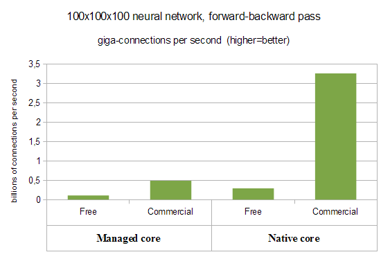
With managed core we have almost linear speed-up from multithreading (4.6x improvement over Free Edition), but native core delivers really striking results. It shows more than 11x improvement over Free Edition (4.4x from multithreading combined with 2.6x from vectorization).

Futhermore, above we compared managed core with managed one (Free vs Commercial), native core with native one. However, if we compare worst performer (Free Edition, managed core, 0.1 gigaconnections per second) with best one (Commercial Edition, native core, 3.3 gigaconnections per second), we will get even more striking difference in processing speed - more than 30x!

Test 2: single-threaded performance

In previous test we used everything from vectorization to multithreading. It is really interesting to compare different ALGLIB editions in "maximum performance" mode. However, it is also interesting to compare single-threaded performance of managed code, generic C code and SSE-capable one.

Here "managed code" corresponds to C# core, either Free Edition - or commercial one, but used in single-threaded mode; "generic C" is C++ core, Free Edition - or commercial one in single-threaded mode and compiled without SSE support; "SSE-capable" is a Commercial Edition compiled with SSE-support.

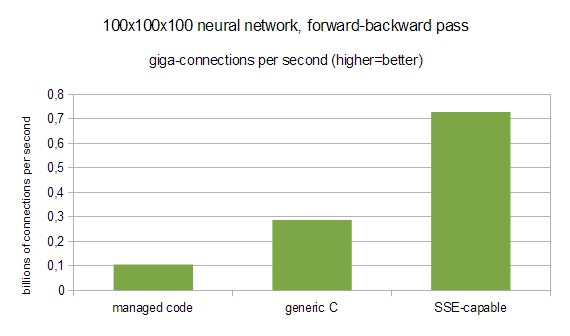
You may see that simply moving from C# to C/C++ gives us about 2.7x performance boost, but turning on SSE support gives additional 2.5x increase in performance. If we compare best performer (Commercial Edition, native core) with worst one (managed core), we will see that difference is even more pronounced - up to 7x!

Test 3: multicore scaling

In this test we'll study how performance of Commercial Edition scales with number of CPU cores. ALGLIB can parallelize following parts of neural training:

• error function evaluation (forward pass) - large chunks of work can be split between different cores
• gradient evaluation (forward-backward pass) - same as network error
• training with restarts - if you train several network from random initial states (specify NRestarts≥2) in order to choose best one, ALGLIB may train these networks in parallel manner.
• cross-validation - training of networks corresponding to different folds can be parallelized too.

State-of-the-art parallel framework used by ALGLIB can efficiently combine different kinds of parallelism. Say, if you train network on dataset S with 2 random restarts, it means than ALGLIB will create two neural networks NET₁ and NET₂, set random initial states, and train them on S independently. Then, best network will be chosen and returned to you. On 1-core system ALGLIB will train NET₁, then will train NET₂. On 8-core system ALGLIB will train NET₁ on cores 0...3, and NET₂ will be trained on cores 4...7. Dataset S will be split between cores, so each of 4 cores assigned to network will have something to work with. Work stealing is extensively used to ensure almost 100% efficiency.

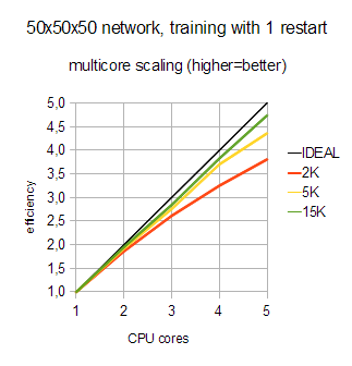
In this test we trained 50x50x50 neural network on datasets of different sizes - from 2.000 to 15.000 samples. Such network has about 5.000 connections, so overall cost of one gradient evaluation varies from 10.000.000 to 75.000.000 connection updates.

First chart (below) shows how multicore training of one network (NRestarts=1) scales with number of cores. Because neural training is a combination of inherently sequential and highly parallel phases, with small samples we should not expect 100% efficiency. But you may see that ALGLIB works well even for small samples (2.000 samples) - it is still beneficial to add more and more cores. However, real efficiency comes with large samples - from 5K to 15K and higher.

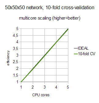
Above we solved "hard" problem - training with moderately-sizes samples and just one restart. Presence of sequential phases in the neural training limits its multicore scaling (Amdahl's law), but still we got good results. But what if we try to solve problem which is inherently parallel? Let's estimate multicore scaling of 10-fold cross-validation on dataset with 15K items.

Cross-validation involves training of ten different (and completely independent) neural networks, so it is easy to parallelize. Furthermore, large dataset size allows us to parallelize gradient evaluation, which is helpful at the last stages of cross-validation, when there are only one or two neural networks left untrained.

From the chart below you may see that efficiency is striking - almost 100%! We have not performed this test on system with larger number of cores, but another data we have at hand allow us to conclude that ALGLIB scales well up to tens of cores, assuming that neural network fits into per-core cache.

This article is licensed for personal use only.