Spline interpolation and fitting

Cubic spline interpolation/fitting is a fast, efficient and stable method of function interpolation/approximation. ALGLIB package provides you with dual licensed (open source and commercial) implementation of spline-related functionality in several programming languages, including our flagship products:

• ALGLIB for C++, a high performance C++ library with great portability across hardware and software platforms
• ALGLIB for C#, a highly optimized C# library with two alternative backends: a pure C# implementation (100% managed code) and a high-performance native implementation (Windows, Linux) with same C# interface

Our implementation of cubic splines is well tested and has following distinctive features (see below for more complete discussion):

• all popular spline types (linear, cubic, monotone, Hermite, Akima, Catmull-Rom)
• rich functionality (interpolation, derivatives, integration, transformation)
• support for penalized regression spline fitting (linear least squares)
• algorithmic and low-level optimizations, including SIMD-capable code for "heavy" least squares fitting functions

Spline types

Linear spline

The linear spline is just a piecewise linear function. The linear splines have low precision, it should also be noted that they do not even provide first derivative continuity. However, in some cases, piecewise linear approximation could be better than higher degree approximation. For example, the linear spline keeps the monotony of a set of points.

Hermite spline

The cubic Hermite spline is a third-degree spline, whose derivative has given values in nodes. For each node not only the function value is given, but its first derivative value too. Hermite's cubic spline has a continuous first derivative, but its second derivative is discontinuous. The interpolation accuracy is much better than in the piecewise linear case.

Catmull-Rom spline

Catmull-Rom spline is a Hermite spline whose derivatives are chosen to be

Catmull-Rom spline is continuous up to the first derivative; second derivative is discontinuous. It is local: spline values depend only on four function values (two on the left of x, two on the right). It supports two kinds of boundary conditions:

• Parabolically terminated spline. In this case, the boundary interval is represented as the second (instead of the third) degree polynomial (for inner intervals, third-degree polynomials are still used). In a number of cases this provides better accuracy than natural boundary conditions.
• Periodic boundary conditions (this kind of conditions is used to model periodic functions).

Cubic spline

All splines considered on this page are cubic splines - they are all piecewise cubic functions. However, if someone says "cubic spline", they usually mean a special cubic spline with continuous first and second derivatives. The cubic spline is given by the function values in the nodes and derivative values on the edges of the interpolation interval (either of the first or second derivatives).

• If the exact values of the first derivative in both boundaries are known, such spline is called clamped spline, or spline with exact boundary conditions. This spline has interpolation error O(h⁴).
• If the value of the first (or second) derivative is unknown, we can set the so-called natural boundary conditions S''(A)=0, S''(B)=0. Thus, we get a natural spline. The natural spline has interpolation error O(h²). The closer to the boundary nodes the more the error becomes. In the inner nodes the interpolation accuracy is much better.
• One more boundary condition which we can use when boundary derivatives are unknown is the "parabolically terminated spline". In this case, the boundary interval is represented as the second (instead of the third) degree polynomial (for inner intervals, third-degree polynomials are still used). In a number of cases this provides better accuracy than natural boundary conditions.
• We can also set periodic boundary conditions (this kind of conditions is used to model periodic functions).

At last, we can combine different types of boundary conditions for different boundaries. It does make sense if we have only partial information about the function behavior at the boundaries (e.g., we know the left boundary derivative, and have no information about the right boundary derivative).

Akima spline

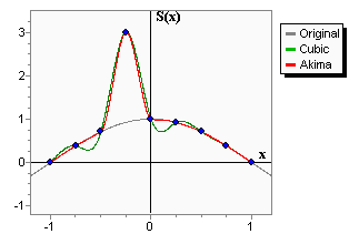
The Akima spline is a special spline which is stable to the outliers. The disadvantage of cubic splines is that they could oscillate in the neighborhood of an outlier. On the graph you can see a set of points having one outlier. The cubic spline with boundary conditions is green-colored. On the intervals which are next to the outlier, the spline noticeably deviates from the given function - because of the outlier. Akima spline is red-colored. We can see that in contrast to the cubic spline, the Akima spline is less affected by the outliers.

An important property of the Akima spline is its locality - function values in [x_i, x_i+1] depends on f_i-2, f_i-1, f_i, f_i+1, f_i+2, f_i+3 only. The second property which should be taken into account is the non-linearity of the Akima spline interpolation - the result of interpolation of the sum of two functions doesn't equal the sum of the interpolations schemes constructed on the basis of the given functions. No less than 5 points are required to construct the Akima spline. In the inner area (i.e. between x₂ and x_N-3 when the index goes from 0 to N-1) the interpolation error has order O(h²).

Monotone spline

Monotone cubic interpolation is a variant of cubic spline that preserves monotonicity of the data being interpolated.

Spline interpolation in ALGLIB

Spline construction

Spline construction is performed using one of the functions below. The result is a spline1dinterpolant structure containing the spline model:

• spline1dbuildlinear - builds linear spline
• spline1dbuildcubic - builds cubic spline
• spline1dbuildhermite - builds Hermite spline
• spline1dbuildakima - builds Akima spline
• spline1dbuildcatmullrom - builds Catmull-Rom spline
• spline1dbuildmonotone - builds monotone cubic spline

Interpolation, differentiation, integration, transformation

After spline is built and you have spline1dinterpolant structure, you can use following functions:

• spline1dcalc - to evaluate spline value at given point
• spline1ddiff - to evaluate spline value and its derivatives at given point
• spline1dintegrate - to integrate spline
• spline1dlintransx - to make linear change of variables x=a·t+b
• spline1dlintransy - to apply linear transformation to spline S₂(x)=a·S(x)+b
• spline1dunpack - to get spline coefficients

Fast batch interpolation on a grid

Conversion from one grid to another is one of the frequently encountered problems involving cubic splines. We have old grid x and function values y (on x) and new grid x₂. We want to calculate function values on a new grid x₂ using cubic splines. Additionally, we may need first or second derivatives.

We can solve this problem by building cubic spline with spline1dbuildcubic function and calling spline1ddiff for each of the new nodes (see below). Such code has O(n₂·log(n₁)) complexity. However, there is an easier and faster solution - to use special functions for grid operations:

• spline1dconvcubic, which calculates cubic spline values on the new grid
• spline1dconvdiffcubic, which calculates cubic spline values and first derivatives on the new grid
• spline1dconvdiff2cubic, which calculates cubic spline values and first/second derivatives on the new grid
• spline1dgriddiffcubic, which differentiates cubic spline on the old grid
• spline1dgriddiff2cubic, which differentiates cubic spline on the old grid (it returns both first and second derivatives)

These functions use algorithm which creates specialized representation of a cubic spline. This representation is optimized for only one kind of operations: conversion/differentiation. It allows to increase performance on presorted grids to O(max(n₂,n₁)).

Note #1
If grids are not presorted, complexity increases to O(n₂·log(n₂)+n₁·log(n₁)) because of time needed to sort grids. However, it is still beneficial to use specialized functions.

Cubic spline fitting

ALGLIB package supports curve fitting using penalized regression splines. Fitting by penalized regression splines can be used to solve noisy fitting problems, underdetermined problems, and problems which need adaptive control over smoothing. It is one of the best one dimensional fitting algorithms. If you need stable and easy to tune fitting algo, we recommend you to choose penalized splines.

This functionality is described in more details in the corresponding chapter of ALGLIB User Guide.

Examples

ALGLIB Reference Manual includes following examples on cubic spline interpolation:

• spline1d_d_linear - shows how to build/use linear spline
• spline1d_d_cubic - shows how to build/use cubic spline with different boundary conditions
• spline1d_d_griddiff - shows differentiation on a grid
• spline1d_d_convdiff - shows conversion from one grid to another

Numerical results

In this section we will show numerical results obtained from solution of different problems. We will investigate following "typical" problems:

• interpolatiopn of a smooth function. Accuracy achieved with different spline types is demonstrated.

Interpolation by different spline types

Consider the following problem: interpolation of f(x)=sin(x) on [-π/2,+π/2]. We use equidistant grid with N nodes and four different types of cubic splines:

• Catmull-Rom spline
• cubic spline with natural boundary conditions
• parabolically terminated cubic spline
• cubic spline with exact boundary conditions (we know exact value of derivative at boundary point)

Having investigating dependency of interpolation error on number of nodes, we can get following chart:

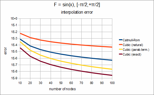
We can see that in this case the best choise is to use cubic spline with exact boundary conditions. If we don't know derivative value at boundary points, we can use cubic spline with exact boundary conditions and get slightly worse results. Other choices - Catmull-Rom spline and cubic spline with natural boundary conditions - give us significantly larger interpolation error.

This conclusion holds true in most cases. If you know derivative at the boundary, use it. If you don't - use parabolically terminated spline.

Note #2
We didn't show results for Hermite spline on the chart above. Usually it gives results similar to spline with exact boundary conditions, but requires more information.

This article is licensed for personal use only.