The rational interpolation (i.e. interpolation by rational functions) consists of the representation of a given function as the quotient of two polynomials:
Parallel with the spline interpolation spline interpolation, the rational interpolation is an alternative for the polynomial interpolation. The main disadvantage of the polynomial interpolation is that it is unstable on the most common grid - equidistant grid. If we are free to choose the grid, we can solve the problem by choosing the Chebyshev nodes. Otherwise (or if we just need a less node-dependent algorithm) the rational interpolation can be an appropriate alternative for the polynomial interpolation.
1 History: first rational interpolation algorithms
2 History: first barycentric algorithms
3 Floater-Hormann algorithm: interpolation without poles
4 Floater-Hormann algorithm: selecting d
5 Barycentric models: construction using coefficients
6 Barycentric models: interpolation
7 Barycentric models: fitting
8 Barycentric models: evaluation/differentiation
9 Barycentric models: other operations
10 Links
11 Downloads section
The rational interpolation is one of the most difficult methods of interpolation. Its advantages are the high accuracy and absence of the problems which are typical for polynomial interpolation. At the same time, these methods have several weaknesses: for example, we can always find an interpolating polynomial for any set of points, but not all set of points have an interpolating rational function. Poles are also a big problem. They tend to appear unexpectedly. However, the last methods can solve most of the problems typical for the first rational interpolation methods. To make this clear, it is worth considering the evolution of rational interpolation algorithms.
One of the first methods for constructing the rational interpolant was by solving a set of equations in unknown coefficients of polynomials p(x) and q(x) (numerator and denominator respectively). However, if the number of points is too large, the set of equations will be ill-conditioned and the coefficients will be calculated with considerable errors. Generally, errors always exist when calculating coefficients. Even small errors could cause the fact that the rational interpolant will not pass through all given points. That's why this algorithm is not applied in practice.
To solve this problem, Bulirsch and Stoer suggested Neville's algorithm generalization for the case of rational interpolation. Bulirsch-Stoer algorithm constructs the rational function by having numerator and denominator degrees equal to N/2 (you can find a detailed description in Numerical Recipes in C [1]). This algorithm has two disadvantages which prevent it from practical usage. First, there are sets of points which the interpolant cannot be constructed for, thus, the algorithm can't detect such cases. Secondly, there is no mechanism to find the poles. It is specific for the rational interpolation that even if the function to be interpolated doesn't have any poles, the interpolant could have unknown numbers of poles in unknown points. Bulirsch-Stoer algorithm can't detect the poles in an interpolation interval.

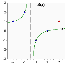
There is a a little artificial example demonstrating both disadvantages in the diagram above. The graph has 5 points: x = [-2, -1, 0, 1, 2], y = [1, 2, -1, 0, 1]. On the basis of these points, the rational interpolant was constructed as having a numerator and a denominator of second degree (the very same interpolant would be constructed by using the Bulirsch-Stoer algorithm). The interpolant has a pole in x = -0.5 although we can't say that the function to be interpolated has poles. Also, the interpolating function doesn't pass through one of the points, just because there is no function with second degree numerator and denominator which can pass through all points. None of these problems could be detected automatically by using the Bulirsch-Stoer algorithm.
The Bulirsch-Stoer algorithm was the only practical algorithm for rational interpolation for a long time. Even now many numerical analysis specialists don't know about the latest achievements in this area. In 1986, C. Schneider and W. Werner published an article where the new rational interpolation algorithm was described. This algorithm used the barycentric representation of a rational interpolant:

If we choose the barycentric weights wj by using the Schneider-Werner algorithm, the expression above becomes a rational function with the required M-th degree denominator (and (N-M)-degree numerator). This algorithm not only constructs rational interpolant in barycentric form, but can test whether poles and unattainable points exist in it. Later on, this algorithm was improved by Berrut and others (see 'Recent developments in barycentric rational interpolation', Jean-Paul Berrut, Richard Baltensperger and Hans D. Mittelmann, 2005 [2]).
The algorithm suggested by Berrut and others solves almost all problems which prevent the Burlisch-Stoer algorithm from practical usage. Unfortunately, new problems appeared. When N and M increase, the problem conditionality becomes worse which causes increasing of wj error and inauthenticity of conclusions about poles and unattainable points. Thus, the algorithm reliability and stability are not good enough to recommend it as the universal solution.
Almost at the same time, an article was published by Floater and Hormann [3], where the algorithm for constructing the interpolating function without poles was described. The Floater-Hormann algorithm is fast, stable and reliable. In many aspects, it can be compared with spline interpolation. The algorithm is described in detail in the article which can be downloaded from the site of one of the authors. Here we will give a short description of it.
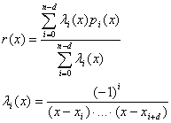
Given points x0, ..., xN and function values in them fi = f(xi). Let d - degree of Floater-Hormann interpolation scheme (0 ≤ d ≤ n) and let pi(x) be a polynomial interpolating f in points xi, ..., xi+d. Then, the Floater-Hormann rational interpolant r(x) is defined as

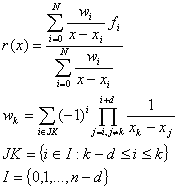
The above formula for r(x) gives an understanding of d, but it is not applicable because of its high calculation complexity. The barycentric formula is faster and more convenient:

Such function r(x) has some important characteristics. First, this function is a rational function having degrees of numerator and denominator not more than N. Second, it has no poles on real axis. Third, if h = max(xi-xi-1), the approximation error has an order of O(hd+1). In some sense, Floater-Hormann interpolation is related to general rational interpolation like a spline interpolation is related to general polynomial interpolation algorithm.
d defines the interpolating scheme power and, consequently, its accuracy. It seems that the bigger d we choose, the less interpolation error we will get, but this effect has an upper bound. The following tables compare the interpolation error for different N and d on equidistant grids on interval [-5;5]. f = sin(x) and f = 1/(1+x2) are used for comparison (a similar analysis was performed in Floater and Hormann's article).
f=sin(x)
N     D=3       D=5       D=8       D=N       Optimal D
 10   1.28e-02  5.21e-03  1.62e-03  6.30e-03  1.62e-03 (D=8)
 20   1.23e-03  1.26e-04  1.96e-05  1.72e-09  1.72e-09 (D=19)
 40   8.47e-05  3.17e-06  3.03e-08  9.53e-07  2.45e-13 (D=15)
 80   5.42e-06  5.50e-08  3.46e-11  2.05e+03  3.24e-14 (D=12)
160   3.39e-07  8.85e-10  4.00e-14  1.48e+02  2.78e-15 (D=10)


f=1/(1+x^2) (Runge example)
N     D=3       D=5       D=8       D=N       Optimal D
 10   6.91e-02  2.42e-01  1.41e+00  1.92e+00  3.61e-02 (D=0)
 20   2.83e-03  9.94e-03  7.04e-02  5.98e+01  1.54e-03 (D=1)
 40   4.31e-06  1.82e-05  1.30e-04  1.05e+05  4.31e-06 (D=3)
 80   5.12e-08  7.98e-10  4.54e-10  1.31e+10  2.03e-10 (D=7)
160   2.98e-09  1.14e-11  8.25e-15  4.57e+01  1.67e-15 (D=11)
The first function is well interpolated by the usual polynomials. The rational interpolation also works well with moderate values of d. Starting from some value of d the error tends to increase, so the optimal value of d belongs to an interval from 8 to 20. Floater and Hormann show that the accuracy of the interpolational scheme usually is not worse than the accuracy of cubic splines.
Runge's function is the classical example of a function which cannot be interpolated by a polynomial on an equidistant grid. Floater-Hormann's rational interpolation solves this problem. By comparing the interpolating accuracy, we can note that the optimal d is less than the optimal d for f = sin(x).
It is interesting how the error behaves when d is rather big, specifically - equal to N. The error increases, sometimes it could be very big (up to 1010). The analysis which was performed using high precision arithmetics showed that in infinite precision arithmetics the error decreases while d increases. However, in finite precision arithmetics, if d is close to N, floating point errors ruin the accuracy of the interpolation scheme. When 3 ≤ d ≤ 8, the interpolating function is calculated with close to machine precision.
To sum up all that is stated above, we can formulate rules for choosing d. If high interpolation precision is required and there is an appropriate possibility, you should choose an optimal d which provides minimal error. If it's impossible to choose optimal d, you should select it from 3 to 8. d = 3 is rather good for both cases, so you can use this as a default value. For example, d = 8 is much better than d = 3, if you have to interpolate "good functions" like sine/cosine, and worse if you interpolate functions like Runge's function. Thus, if we don't know what class of functions our function belongs to, it's better to choose d = 3.
Barycentric model can be built from points xi/yi and weights wi provided by user. This task is solved by barycentricbuildxyw function. Its result is barycentricinterpolant stucture, which may be used with other subroutines of ratint unit - to evaluate function at some point, to differentiate rational function, etc.
barycentricbuildfloaterhormann function builds barycentric interpolant using Floater-Hormann algorithm. Algorithm inputs are points xi/yi and d parameter, its result is barycentricinterpolant structure again.
ALGLIB library supports rational fitting using Floater-Hormann basis functions. barycentricfitfloaterhormann subroutine solves unconstrained task without individual weights. barycentricfitfloaterhormannwc subroutine solves more complex task: constrained fitting (C suffix) with individual weights (W suffix). Arbitrary number of constraints on function value - f(xc)=yc - or its derivative - df(xc)/dx=yc - is supported.
Note #1
Excessive constraints may be inconsistent, especially when you work with simple models. See Reference manual, barycentricfitfloaterhormannwc comments, for more information on this subject.
Both subroutines use Floater-Hormann basis built on equidistant grid with M nodes. They search for optimal D in [0,9] ("optimal" means "least weighted RMS error"). Because such fitting task is linear, Linear Least Squares solver with O(N·M2) complexity is used (here N is a number of points, M is a basis size).
It is important to note that reduced set of rational functions is used for fitting - set of Floater-Hormann rational functions, which have no poles on the real axis. From the one side, Floater-Hormann basis is more stable. From the other side, Floater-Hormann functions have less degrees of freedom than general rational function - hence less precision. You may achieve error as small as 10-3...10-5 using only moderate number of points. But interpolation/fitting error have geometric, not exponential convergence, so Floater-Hormann function are not well suited for tasks where extra high precision with limited number of points is needed.
After the rational function is built,barycentriccalc may be used to evaluate rational function. If you want to calculate first/second derivatives, you may use barycentricdiff1 and barycentricdiff2 subroutines.
Other operations include:
This article is licensed for personal use only.
ALGLIB Project offers you two editions of ALGLIB:
ALGLIB Free Edition:
+delivered for free
+offers full set of numerical functionality
+extensive algorithmic optimizations
-no multithreading
-non-commercial license
ALGLIB Commercial Edition:
+flexible pricing
+offers full set of numerical functionality
+extensive algorithmic optimizations
+high performance (SMP, SIMD)
+commercial license with support plan
Links to download sections for Free and Commercial editions can be found below:


