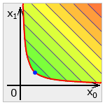
Nonlinearly constrained solver

Nonlinearly constrained optimization is an optimization of general (nonlinear) function subject to nonlinear equality and inequality constraints.

It is one of the most esoteric subfields of optimization, because both function and constraints are user-supplied nonlinear black boxes. Many techniques which worked with linear constraints do not work now - say, it is impossible to handle constraints analytically, like it was done in BLEIC optimizer.

Most nonlinear optimizers are hard to use and tune. However, we tried to provide you state-of-the-art nonlinear solvers which do not require extensive tuning. This article discusses these solvers and their properties.

Note #1
This article complements ALGLIB Reference Manual - a technical description of all ALGLIB functions with automatically generated examples. If you want to know what functions to call and what parameters to pass, Reference Manual is for you. Here, in ALGLIB User Guide, we discuss ALGLIB functionality (and optimization in general) in less technical manner. We discuss typical problems arising during optimization, mathematical algorithms implemented in ALGLIB, their strong and weak points - everything you need to get general understanding of nonlinearly constrained optimization.

Nonlinearly constrained optimization overview

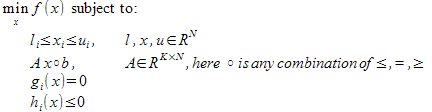
Barrier/penalty methods were among the first ones used to solve nonlinearly constrained problems. The idea is simple: if you want to solve constrained problem, you should prevent optimization algorithm from making large steps into constrained area (penalty method) - or from crossing boundary even just a bit (barrier method). The most natural way to do so is to modify function by adding penalty or barrier term (see chart below).

You may see that both methods work, but they are unable to find solution with high precision. Either they "overshoot" (penalty method, which stops at infeasible point) or "undershoot" (barrier method, which stops at some distance from the boundary). This limitation can be partially overcome by making barrier/penalty term "sharper", which increases precision. But additionally it results in increased condition number - and increased number of iterations required to solve problem.

Several approaches have been developed to combat limitations of barrier/penalty methods. One of such solutions is augmented Lagrangian method, which combines penalty term which special adjustable shift term. When you stop behind the boundary, shift term is adjusted in such way that next outer iteration of AUL algorithm will move you back to feasible area. Thus, augmented Lagrangian optimization algorithm uses inner-outer iteration schema, when a sequence of inner iterations with fixed values of meta-parameters (coefficients of shift term) forms one outer iteration. In most cases you will need from 2 to 10 outer iterations to achieve good precision.

Strong sides of augmented Lagrangian algorithm are its precision and speed (when compared with barrier/penalty methods). From the other side, outer iteration requires very tight stopping criteria for inner iterations! Update algorithm for shift term requires us to stop close to extremum of modified merit function (target function + penalty term + shift term). If you stop too far from the extremum, update algorithm for shift term may be destabilized. In this case algorithm will perform random oscillation around true solution, with precision even worse than that of barrier/penalty algorithm!

Note #2
First outer iteration of augmented Lagrangian algorithm is equivalent to barrier/penalty method, because it is performed with zero shift term. So if you need quick and dirty (but stable!) solution, you may often get find good one with just one outer iteration!

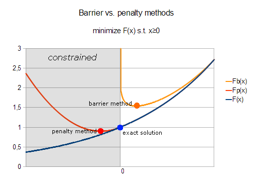
There are many approaches to nonlinearly constrained optimization. Although almost all of them include some form of penalty or barrier term, there are still exist differences in the way algorithms make use of this term. Augmented Lagrangian algorithm is only one of such algorithms. One alternative approach is to use non-smooth penalty, also known as L1 penalty.

L1 penalty takes form ρ·|g_i(x)| for equality constraint g_i(x)=0, and it is equal to ρ·max(h_i(x),0) for inequality constraint h_i(x) ≤ 0. Such penalty is an exact one, i.e. for sufficiently large ρ exact solution of penalized problem is equal to exact solution of original constrained problem (see chart above).

One pretty obvious drawback of such approach is that you move from constrained optimization to nonsmooth optimization. Both kinds of optimization problems are hard to solve - mathematically hard and computationally hard. However, sometimes nonsmooth problems are computationally hard - but easy in any other respect. Say, gradient sampling algorithm requires lots of function evaluations, but works robustly and does not require fine-tuning. So, if you have low-dimensional problem, lots of computational time - but do not want to spend too much of your personal time, L1-penalized optimization is a good way to go.

NLC solvers provided by ALGLIB

AUL solver

AUL (AUgmented Lagrangian) solver is provided by minnlc subpackage of Optimization package. AUL solver includes several important features:

• special handling of box/linear constraints
• variable scaling (in order to handle badly scaled problems)
• two kinds of preconditioners - approximate LBFGS-based one or exact low-rank one
• built-in support for numerical differentiation

There are several limitations of AUL solver you should know about, though. First, this solver requires that nonlinear constraints g_i and h_i satisfy particular requirements (so called constraint qualification): they must have non-zero gradient at the boundary. Say, constraint like x²≤1 is supported, but x²≤0 is very likely to confuse optimizer. Furthermore, it is required that there exists inner point, i.e. point where all inequality constraints are strictly less than zero. E.g. combination of constraints x≤0 and -x≤0 may destabilize optimizer (such pair of constraints should be replaced by one equality constraint).

Another important limitation is AUL solver is optimized for moderate amount of non-box (nonlinear or general linear) constraints. Hundreds of linear/nonlinear constraints are OK, but thousands may make optimization process too slow.

AGS solver

AGS (Adaptive Gradient Sampling) solver is provided by minns subpackage of Optimization package. This solver is intended for solution of nonsmooth problems with box, linear and nonlinear (possibly nonsmooth) constraints. AGS solver includes several important features:

• special handling of box/linear constraints
• variable scaling (in order to handle badly scaled problems)
• built-in support for numerical differentiation

The most important limitation of AGS solver is that this solver is SLOW and not intended for high-dimensional problems. One AGS step requires ~2·N gradient evaluations at randomly sampled locations (just for comparison - LBFGS requires O(1) evaluations per step). Typically you will need O(N) iterations to converge, which results in O(N²) gradient evaluations per optimization session.

Furthermore, if you use numerical differentiation capabilities provided by AGS solver, you will need ~4·N² evaluations per step, and O(N³) function evaluations per session.

Finally, this method has convergence speed of steepest descent (when measured in iterations, not function evaluations). The only practical difference from steepest descent is algorithm's ability to handle nonsmooth problems and box/linear/nonlinear constraints.

From the other side, this solver requires only a little tuning. Once you select initial sampling radius (almost any sufficiently large value will work) and penalty parameter for nonlinear constraints, it will be working like a bulldozer - slowly but robustly moving towards solution. Algorithm is very tolerant to its tuning parameters, so you won't have to make numerous trial runs in order to find good settings for your optimizer.

Solving nonlinearly constrained problems with ALGLIB

minnlcstate and minnsstate objects

As all ALGLIB optimizers, minnlc unit is built around minnlcstate object. You should use it for everything optimization-related - from problem specification to retrieval of results:

1. create instance of optimizer with minnlccreate (or minnlccreatef - for numerical differentiation) function
2. choose one of the optimization algorithms by means of appropriate function (as for now, only one solver, AUL, is present, which is activated by minnlcsetalgoaul call)
3. pass to optimizer problem specifications like box/linear constraints, scale of variables, number of nonlinear constraints
4. start optimizer with minnlcoptimize function
5. retrieve results with minnlcresults function

You should work with minns unit in a similar way:

1. create instance of optimizer with minnscreate (or minnscreatef - for numerical differentiation) function
2. choose one of the optimization algorithms by means of appropriate function (as for now, only one solver, AGS, is present, which is activated by minnssetalgoags call)
3. pass to optimizer problem specifications like box/linear constraints, scale of variables, number of nonlinear constraints
4. start optimizer with minnsoptimize function
5. retrieve results with minnsresults function

Choosing between analytic and exact gradient

Before starting to use AUL/AGS optimizers you have to choose between numerical diffirentiation or calculation of analytical gradient. For example, if you want to minimize f(x,y)=x²+exp(x+y)+y², then optimizer will need both function value at some intermediate point and function derivatives df/dx and df/dy. How can we calculate these derivatives? ALGLIB users have several options:

1. gradient is calculated by user, usually through symbolic differentiation (so called analytical or exact gradient). This option is the best one because of two reasons. First, precision of such gradient is close to the machine ε (that's why it is called exact gradient). Second, computational complexity of N-component gradient is often only several times (not N times!) higher than calculation of function itself (knowledge of the function's structure allows us to calculate gradient in parallel with function calculation).
2. gradient is calculated by ALGLIB through numerical differentiation, using 4-point difference formula (AUL solver) or 2-point one (AGS solver). In this case user calculates function value only, leaving all differentiation-related questions to ALGLIB package. This option is more convenient than previous one because user don't have to write code which calculates derivative. It allows fast and easy prototyping. However, we can note two significant drawbacks. First, numerical gradient is inherently inexact (even with 4-point differentiation formula), which can slow down algorithm convergence. Second, numerical differentiation needs 4·N function evaluations in order to get just one gradient value. Thus numerical differentiation will be efficient for small-dimensional (tens of variables) problems only. On medium or large-scale problems algorithm will work, but very, very slow.

Depending on the specific option chosen by you, you will use different functions to create optimizer and start optimization - minnlccreate/minnscreate for user-supplied gradient, minnlccreatef/minnscreatef for numerical differentiation provided by ALGLIB.

You should also pass corresponding callback to minnlcoptimize/minnsoptimize - one which calculates function and gradient for the former case, one which calculates function vector only for the latter case. If you erroneously pass callback calculating function value only to optimizer structure created with minnlccreate/minnscreate, then optimizer will generate exception on the first attempt to use gradient. Similarly, it will generate exception if you pass callback calculating gradient to optimizer object which expect only function value.

Scale of the variables

Before you start to use optimizer, we recommend you to set scale of the variables with minnlcsetscale/minnssetscale functions. Scaling is essential for the correct work of the stopping criteria (and sometimes for the convergence of optimizer). You can use optimizer without scaling if your problem is well scaled. However, if some variables are up to 100 times different in magnitude, we recommend you to tell solver about their scale. And we strongly recommend to set scaling in case of larger difference in magnitudes.

We recommend you to read separate article on variable scaling, which is worth reading unless you solve some simple toy problem.

Tuning AUL solver

Augmented Lagrangian solver is one of the fastest nonlinearly constrained optimization algorithms, but it requires careful tuning. First, you should carefully select stopping criteria for inner iterations, which are set with minnlcsetcond function. Second, you should carefully tune outer iterations of the algorithm.

One distinctive trait of augmented Lagrangian method is that it requires very stringent stopping criteria for inner iterations. Lagrange multipliers are updated using information about constraint violation at the end of the previous outer iteration. Thus, you should solve previous optimization subproblem very precisely in order to get good update for the next one. We recommend you to use step length as stopping condition, and to use very small lengths, like ε_x=10^-9 or smaller.

There are two parameters which control outer iterations of the algorithm: penalty coefficient ρ and number of outer iterations ItsCnt. We strongly recommend you to read comments on minnlcsetalgoaul function, sections named "HOW TO CHOOSE PARAMETERS", "SCALING OF CONSTRAINTS" and "WHAT IF IT DOES NOT CONVERGE?". These sections summarize our experience with the algorithm.

Tuning AGS solver

AGS (Adaptive Gradient Sampling) solver is a good option for situations when you solve moderately-sized problem (from several to tens of variables) and all you need is just a robust solver which does not require difficult tuning with multiple trial-and-error attempts. Such simplicity has only one drawback - like all gradient sampling methods, AGS is slow and requires really many function evaluations.

Examples

• minnlc_d_mixed - an example which demonstrates application of MinNLC solver to mixed nonlinear equality/inequality constraints
• minns_d_nlc - an example which demonstrates application of MinNS solver to mixed nonlinear equality/inequality constraints

This article is licensed for personal use only.